
Computing QR Decomposition with Householder Vectors
February 25, 2025 · 11 min readAs I’ve discussed in a previous post, I have been working through my own C++/Python implementation of the CSparse routines from Tim Davis’s SuiteSparse package, as described in his book. In Chapter 5 of the book, he describes how to compute the QR decomposition of a sparse matrix using Householder reflections. As I work through the implementation, I test my code against output from MATLAB and SciPy. I noticed a difference in output between the code presented in Davis’s book and the code used internally by MATLAB and SciPy. In this post, I explore the differences between the two methods.
Householder Reflections
A Householder reflection is a linear transformation that reflects a vector across a plane defined by its normal vector. In this context, we use Householder reflections to find an orthogonal basis for the column space of a matrix, which is the basis for the QR decomposition.
The Householder reflection is defined as
\[H = I - \beta v v^T\]where $I$ is the identity matrix,
\[\beta = \frac{2}{v^T v}\]and $v$ is a vector that defines the plane of reflection. It is convenient to normalize $v$ such that $v_1 = 1$, or
\[v = \begin{bmatrix} 1 \\ v_2 \\ \vdots \\ v_N \end{bmatrix},\]so that we only need to store the elements $v_2, \ldots, v_N$.
We are interested in finding the Householder vector $v$ that will zero out all elements below the diagonal of a given column of a matrix. We can then apply these steps successively to each column to find the QR decomposition of the matrix, or more directly, the $V$ matrix of Householder vectors, a vector $\beta$ of scaling factors, and the $R$ matrix of the QR decomposition.
The correct Householder vector $v$ will give a reflection matrix that gives
\[Hx = \pm \|x\| e_1\]when applied to a vector $x$, where $e_1$ is the first column of the identity matrix. Figure 1 illustrates the reflection of a vector $x$ across two possible planes onto $e_1$.
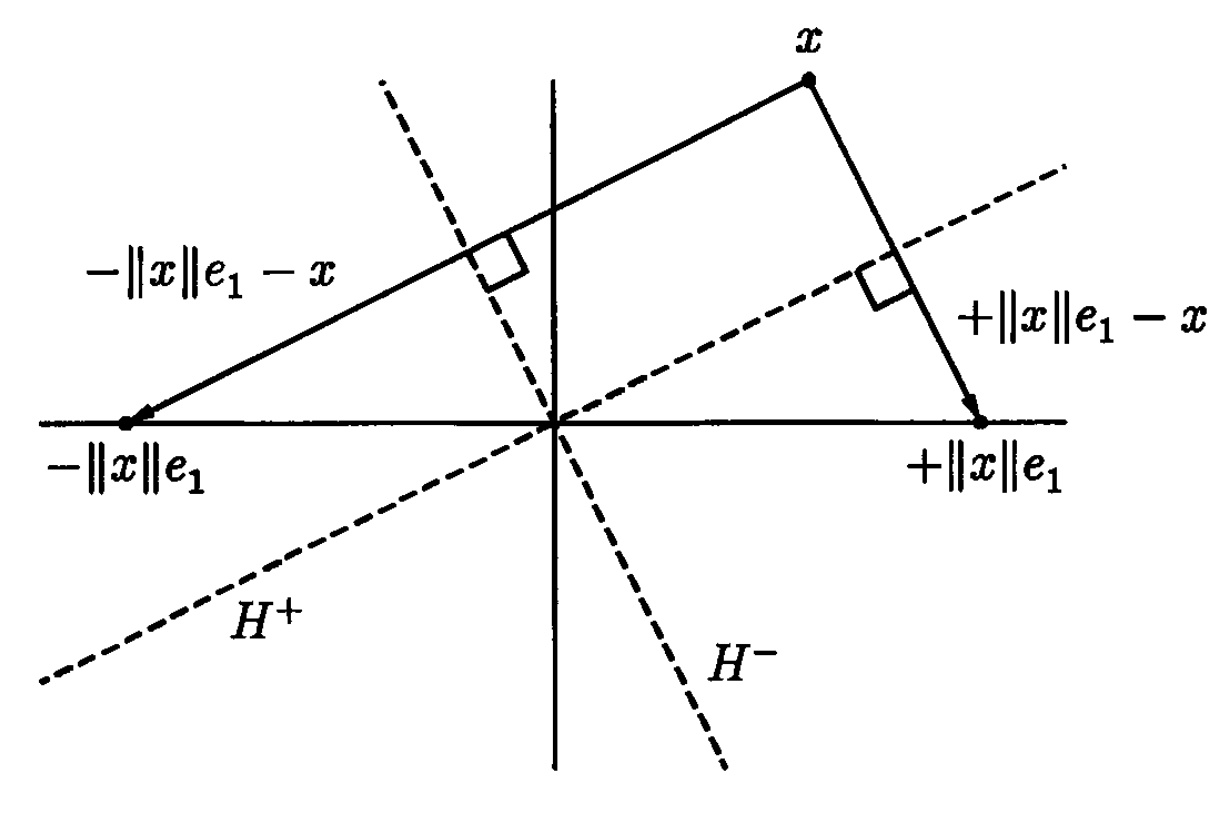
Figure 1. Reproduced from Trefethen and Bau (1997), “Numerical Linear Algebra”, Figure 10.2 (p 72). The Householder reflection $Hx$ of a vector $x$ across two possible planes.
The choice of sign for the reflector is mathematically arbitrary, but this step is where Davis and MATLAB/SciPy differ.
There are two variables (giving four cases) to consider:
- $x$ is already in the direction of a unit vector, i.e. $x = c e_1$ for some scalar $c$, or it is in an arbitrary direction.
- The first element of $x$, $x_1$, is either positive or it is negative.
We will show how Davis and MATLAB/SciPy handle each of these cases, and how their choices affect the numerical properties of the method.
The Davis Method
In the case where $x$ is already in the direction of a unit vector, Davis chooses the sign such that $Hx = +\|x\| e_1$ is always in the positive direction, regardless of the sign of $x_1$. Thus,
\[\begin{align*} v &= \begin{bmatrix} 1 \\ x_2 \\ \vdots \\ x_N \end{bmatrix} \\ \beta &= \begin{cases} 0 & \text{if } x_1 > 0 \\ 2 & \text{otherwise} \end{cases} \end{align*}\]In the case where $x$ is not already in the direction of a unit vector, Davis describes the Householder reflection by
\[\begin{align*} v &= \begin{bmatrix} x_1 - \|x\| \\ x_2 \\ \vdots \\ x_N \end{bmatrix} \\ \beta &= \frac{-1}{\|x\| - v_1} \end{align*}\]When $x_1 > 0$, Davis uses an alternative calculation of $x_1 - |x|$ to avoid cancellation errors:
\[\begin{align*} x_1 - \|x\| &= ( x_1 - \|x\| ) \frac{x_1 + \|x\|}{x_1 + \|x\|} \\ &= \frac{x_1^2 - \|x\|^2}{x_1 + \|x\|} \\ &= \frac{x_1^2 - \left( x_1^2 + x_2^2 + \cdots + x_N^2 \right) }{x_1 + \|x\|} \\ &= \frac{-\|x_2\|^2}{x_1 + \|x\|}. \end{align*}\]The function cs_house presented in the book does not normalize the vector, but
that can be done easily by
and does not otherwise affect the computation.
Davis cites Golub and Van Loan, Algorithm 5.1.1, for the derivation of the Householder reflection. Golub and Van Loan show a slightly different expression for $\beta$, but the two are equivalent.
The LAPACK Method
The method used by MATLAB and SciPy is based on the
LAPACK routine DLARFG.
In the case where $x$ is already in the direction of a unit vector, the routine chooses $\beta = 0$, so that $H = I$, and $Hx = x$, sign included.
In the case where $x$ is not already in the direction of a unit vector, the LAPACK routine chooses
\[\begin{align*} s &= -\text{sign}(x_1) \|x\| \\ v &= x - s e_1 = \begin{bmatrix} x_1 - s \\ x_2 \\ \vdots \\ x_N \end{bmatrix} \\ \beta &= \frac{s - v_1}{s} \\ \end{align*}\]and then normalizes $v$ by dividing by $v_1$. LAPACK’s choice of sign for $s$ follows Trefethen’s convention, which is to reflect $x$ in the direction farthest from $x$ itself.
Visual Comparison
Figure 2 Shows the vectors produced by each method for the input $x = [3, 4]^T$ (so that the norm $\|x\| = 5$).

Figure 2. A comparison of the two methods for an arbitrary vector $x = [3, 4]^T$.
We can see that the Davis method chooses the reflection closest to $x$ (across the $H^+$ plane), while the LAPACK method chooses the reflection farthest from $x$ (across the $H^-$ plane).
We can also compare the two methods for a few more cases:
| $x$ | $v_D$ | $v_L$ | $\beta_D$ | $\beta_L$ | $s_D$ | $s_L$ |
|---|---|---|---|---|---|---|
| [ 3, 0] | [1, 0 ] | [1, 0 ] | 0 | 0 | 3 | 3 |
| [-3, 0] | [1, 0 ] | [1, 0 ] | 2 | 0 | 3 | -3 |
| [ 3, 4] | [1, -2 ] | [1, 0.5] | 0.4 | 1.6 | 5 | -5 |
| [-3, 4] | [1, -0.5] | [1, -0.5] | 1.6 | 1.6 | 5 | 5 |
| [ 3, -4] | [1, 2 ] | [1, -0.5] | 0.4 | 1.6 | 5 | -5 |
| [-3, -4] | [1, 0.5] | [1, 0.5] | 1.6 | 1.6 | 5 | 5 |
The subscript $D$ refers to the Davis method, and $L$ refers to the LAPACK method. The value $s$ is the first element of $Hx$ for the given $x$, $v$, and $\beta$. We can see that Davis always gives a positive $s$, while LAPACK depends on the sign of $x_1$, and whether or not $x$ is in the direction of $e_1$.
While there is no mathematical difference to choosing either reflector, when it comes to the actual numerical computation, there is a major difference in the methods.
Numerical Consequences
To see the numerical consequences of the two methods, we can compare the vector they produce for an input vector that is very close to a unit vector:
\[x = \begin{bmatrix} 1 + \epsilon \\ \epsilon \end{bmatrix}.\]We define the two methods in the following Python functions:
def _house_lapack(x):
    """Compute the Householder reflection vector using the LAPACK method."""
    v = np.copy(x)
    σ = np.sum(v[1:]**2)

    if σ == 0:
        s = v[0]  # if β = 0, H is the identity matrix, so Hx = x
        β = 0
        v[0] = 1  # make the reflector a unit vector
    else:
        norm_x = np.sqrt(v[0]**2 + σ)   # ||x||_2
        a = v[0]
        s = -np.sign(a) * norm_x
        β = (s - a) / s
        # v = x + sign(x[0]) * ||x|| e_1
        # v /= v[0]
        v[0] = 1
        v[1:] /= (a - s)  # a - b == x[0] + sign(x[0]) * ||x||

    return v, β, s


def _house_davis(x):
    """Compute the Householder reflection vector using the Davis method."""
    v = np.copy(x)
    σ = np.sum(v[1:]**2)

    if σ == 0:
        s = np.abs(v[0])           # ||x|| consistent with always-positive Hx
        β = 2 if v[0] <= 0 else 0  # make direction positive if x[0] < 0
        v[0] = 1                   # make the reflector a unit vector
    else:
        s = np.sqrt(v[0]**2 + σ)   # ||x||_2

        # These options compute equivalent values, but the v[0] > 0 case
        # is a more numerically stable option.
        v[0] = (v[0] - s) if v[0] <= 0 else (-σ / (v[0] + s))
        β = -1 / (s * v[0])

        # Normalize β and v s.t. v[0] = 1
        β *= v[0] * v[0]
        v /= v[0]

    return v, β, s
as well as a simple wrapper function that takes method as an argument.
We’ll compute the vector from a “naïve” implementation of the Householder reflection, which does not account for the sign of $x_1$:
import numpy as np
import scipy.linalg as la

ϵ = 1e-15  # a very small number

x = np.r_[1 + ϵ, ϵ]  # a vector very close to e_1 == [1, 0]

# Compute the Householder vector using the naïve method
v = x - la.norm(x)  # cancellation occurs!
with np.errstate(divide='ignore', invalid='ignore'):
    v /= v[0]

# Print the output, ensuring we show small numbers
np.set_printoptions(suppress=False)
print("x:", x)
print("v:")
print("unstable:", v)  # [nan, -inf] divide by zero!

# Show numerical *stability* of the Davis method
v_D, β_D, _ = house(x, method='Davis')
print("   Davis:", v_D)
print(f"     β_D: {β_D:.2g}")

# The LAPACK method is numerically
v_L, β_L, _ = house(x, method='LAPACK')
print("  LAPACK:", v_L)
print(f"     β_L: {β_L:.2g}")
The output is:
x: [1.e+00 1.e-15]
v:
unstable: [ nan -inf]
   Davis: [ 1.e+00 -2.e+15]
     β_D: 5e-31
  LAPACK: [1.e+00 5.e-16]
     β_L: 2
We can see that the unstable method indeed results in cancellation, and the other two methods are stable. Notice that Davis’s method, however, produces a vector whose second element $v_2$ is massive, and whose scaling factor $\beta$ is correspondingly tiny. Constrast this result with the LAPACK method that produces a $v_2 = \frac{\epsilon}{2}$, and $\beta = 2$.
To get a better sense of the trend, we can plot these values vs. $\epsilon$. Figure 3 shows the plot over a broad range of values.

Figure 3. Numerical results for the Householder reflection of a vector that is close to a unit vector for small $\epsilon$, showing the second component of the reflector $v$ and the scaling factor $\beta$.
It turns out that the Davis method follows the trend
\[\begin{align*} v &= \begin{bmatrix} 1, -\dfrac{2}{\epsilon} \end{bmatrix}^T \\ \beta &= \frac{\epsilon^2}{2} \end{align*}\]whereas the LAPACK method is more constained:
\[\begin{align*} v &= \begin{bmatrix} 1, \dfrac{\epsilon}{2} \end{bmatrix}^T \\ \beta &= 2, \end{align*}\]for $\epsilon \ll 1$. In fact, LAPACK guarantees that $\beta = 0$ for $x \propto e_1$, or $\beta \in [1, 2]$ for any other $x$.
For this reason, I have implemented the LAPACK algorithm in my own Householder function.
Householder Vectors in Python and MATLAB
It’s nice to implement our own python functions for transparency, but we can also use built-in SciPy and MATLAB functions to get the same result.
In python:
import numpy as np
import scipy.linalg as la

x = np.r_[3, 4]
(Qraw, β), _ = la.qr(np.c_[x], mode='raw')  # qr input must be 2D
v = np.vstack([1.0, Qraw[1:]])

# Output
>>> v
===
array([[1. ],
       [0.5]])
>>> β
=== array([1.6])
or in MATLAB/Octave: NB: I have only tested this code in Octave. Octave does not normalize the results. I have not tested this code in MATLAB itself.
x = [3, 4]';
[v, beta] = gallery('house', x)

% Note that Octave does *not* normalize the results
% Output
v =

   8
   4

beta = 0.025000

% To match SciPy, run:
>> v1 = v(1);
>> v /= v1
v =

   1.0000
   0.5000

>> beta *= v1^2
beta = 1.6000
Conclusions
We have seen how Householder vectors are defined, and the numerical consequences of two different methods of actually computing their values. This post underlies the importance of numerical stability in algorithms, even when it is not apparent in the underlying mathematical theory.
For a deeper discussion of numerical stability, especially as applied to the Householder version of the QR decomposition, see Trefethen and Bau, Lecture 7 on QR Factorization and Lecture 16 on Stability of Householder Triangularization. Golub and Van Loan Section 5.1 on Householder and Givens Matrices, specifically Algorithm 5.1.1, is the source of much of Davis’s theory. For a more in-depth discussion of the CSparse routines, see Davis, Chapter 5 on Orthogonal Methods.
References
- Davis, Timothy A. (2006). "Direct Methods for Sparse Linear Systems".
- Treftethen, Lloyd and David Bau (1997). "Numerical Linear Algebra".
- Golub, Gene H. and Charles F. Van Loan (1996). "Matrix Computations". 3 ed.